How to Use VLOOKUP Function in a Pivot Table in Excel

VLOOKUP function and PivotTable feature, form a powerful synergy for streamlined data analysis. VLOOKUP, a versatile lookup function, excels at precisely retrieving specific information from vast datasets. When combined with Pivot Tables, which offer dynamic data organization and summarization, these tools become a formidable force in navigating and gaining insights from complex data sets. In this article, I added a step-by-step approach to using VLOOKUP from the Excel Pivot Table. So, let’s start.

Table of Contents Toggle

What is a VLOOKUP Function?

A VLOOKUP function is a powerful tool in spreadsheet software, commonly used in Microsoft Excel and Google Sheets, to search for a specific value in a table and retrieve related information. It stands for “Vertical Lookup” and is particularly useful for large datasets.

Syntax with Explanation of VLOOKUP Function in Excel

The syntax of the VLOOKUP function typically involves four parameters:

=VLOOKUP(lookup_value, table_array, col_index_num, range_lookup)

Lookup Value: The value you want to search for in the first column of the table.
Table Array: The range of cells that contains the data, including the column where the lookup value is located and the columns where you want to retrieve information.
Col Index Num: The column number in the table array from which to retrieve the data. The first column is 1, the second is 2, and so on.
Range Lookup: A logical value indicating whether to find an exact match (FALSE) or an approximate match (TRUE) when searching for the lookup value.

Apply VLOOKUP Function in a Pivot Table in Excel

Dataset to insert Pivot Table for using VLOOKUP form Pivot Table

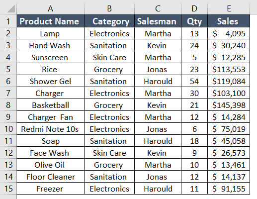
We have a dataset to insert a Pivot Table. Then, I will apply a VLOOKUP formula referring to the Pivot Table.
To create a Pivot Table, select the range and go to Insert tab > PivotTable dropdown > From Table/Range option. Then, confirm the range and location. Now, arrange the Pivot Table.

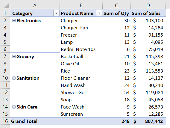
Created Pivot Table dataset to use VLOOKUP function from Pivot Table

In the Pivot Table, we have a sales report summary. There is a list of products with their category. Additionally, the quantity and sales according to each product.
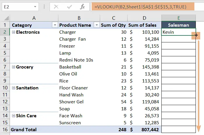
Now, I will add another column to show the names of the salesman from the source data.

To insert a formula with VLOOKUP function, follow the steps below:

Entered formula to use VLOOKUP function from Excel Pivot Table

First, insert a new column and name it.
Copy the formula: =VLOOKUP(B2,Sheet1!A1:E15,3,TRUE)
Paste it into a cell.
Drag it down with the Fill Handle.

Displaying result with VLOOKUP function from Excel Pivot Table

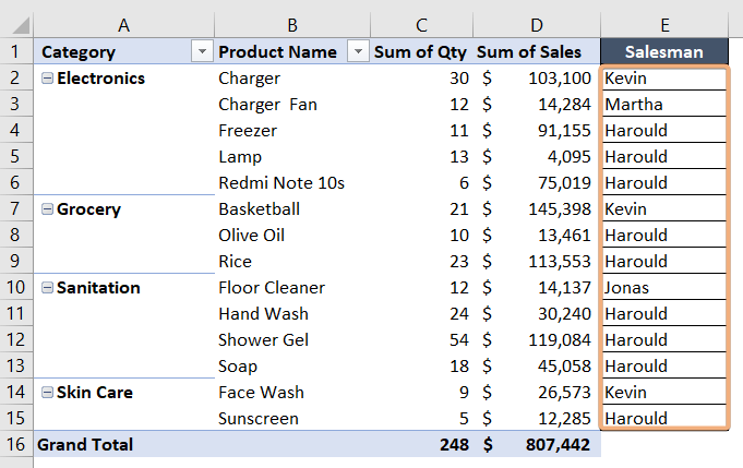
Finally, you will see the names of the salesman in the inserted column using the formula.

Conclusion

In conclusion, the combination of Excel’s VLOOKUP function and PivotTable feature provides a robust toolkit for efficient data analysis and retrieval. VLOOKUP offers a quick and precise way to search for specific values within a dataset, while PivotTables enables dynamic organization and summarization of complex data. In this article, I have provided a guideline to create a VLOOKUP formula from the Pivot Table. Besides, I have explained the basic VLOOKUP formula. So, you can add VLOOKUP from the Pivot Table by going through this article.

Frequently asked questions

What is Pivot formula?

In Excel, the term ‘pivot formula’ does not refer to a specific function but is commonly associated with the creation of pivot tables. Pivot tables are a powerful feature that enables users to dynamically analyze and summarize data. To create a pivot table, select your data, go to the Insert tab, and choose PivotTable. Arrange your data by dragging fields into the Rows and Columns areas, and analyze them by placing fields in the Values area. Understanding how to use the PivotTable tool is essential for efficient data analysis and reporting in Excel.

How do you use the VLOOKUP formula?

To use the VLOOKUP formula in Excel, follow this syntax: =VLOOKUP(lookup_value, table_array, col_index_num, [range_lookup]). Specify the value to search for, the data range, the column number to extract data from, and optionally, whether to allow approximate matches. For example, =VLOOKUP(“ProductA”, A2:C10, 2, FALSE) finds “ProductA” in the first column of A2:C10 and returns the corresponding value from the second column. VLOOKUP is a powerful tool for data analysis and retrieval in Excel, making it easy to extract information from large datasets.

How do you look up data from a Pivot Table?

To look up data from a PivotTable in Excel:

Select the Cell: Click on the cell within the Pivot Table where you want to retrieve data.
Access the Field List: If the Field List is not visible, right-click anywhere in the PivotTable and choose Show Field List.
Drag Field to Rows or Columns: Drag the relevant field from the Field List to either the Rows or Columns area, depending on where it’s located in the Pivot Table.
Review Data: The PivotTable dynamically updates, and you can find the desired data at the intersection of the specified row and column.
Use Filters and Slicers: Further, refine your data by applying filters or using slicers to control the displayed information interactively.

By following these steps, you can easily look up and retrieve specific data points within a Pivot Table in Excel.